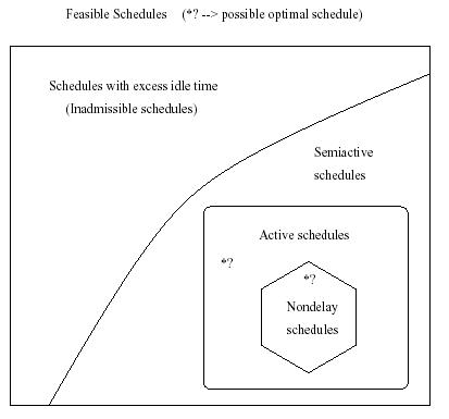
There four kinds of feasible schedules ([8] gives very strict definitions
of feasible and optimal schedules) for a JSSP:
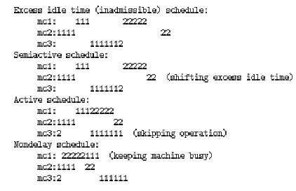
- inadmissible schedules: schedules with excessive idle time.
- semiactive schedules: schedules with no excess idle time.
- active schedules: schedules with no such shifts as by skipping
some oprations to the front without causing other operations to start later
than the original schedule.
- nondelay schedules: in which a machine is never kept idle if some
operation is able to be processes.
The optimal schedule is not necessarily a nondelay schedule but certainly
is an active schedule [5]. The relationship of the four schedules
is as follows[3, 5]:
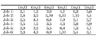
As an example, suppose job1 must go to mc2(machine 2) first, then mc1,
mc3, and job2: mc3, mc1, mc2. We have:
[8] gives 7 steps for calculating all the active schedules with
use of Giffler and Thompson algorithm, which can be interpreted as[3, 5]:
- Calculate the set C of all operations that can be scheduled next;
- Calculate the completion time of all operattions in C, and le
mm equal the machine on which the minimum completion time t is achieved;
- Let G denote the conflict set of operations on machine mm, and
this is the set of operations in C which take place on mm, and whose start
time is less than t;
- Select an operation from G to schedule;
- Delete the chosen operation from C and return to step 1.
As for calculating non-delay schedules, we have [3]:
- Calculate the set C of all operations that can be scheduled next;
- Calculate the starting time of each operation in C and let G equal
the subset of operations that can start earliest;
- Select an operation from G to schedule;
- Delete the chosen operation from C and return to step 1.
The first and most important problem in GA application for JSSP is how to
encode the problem on a chromosome. Among varieties of representations the
most interesting one is "Heuristic Combination Methods (HCM)", like those
in [5, 7, 9]. An implicit representation is used in this method
for a schedule: each gene in a chromosome is a heuristic for each step
of generating a schedule. In following section we introduce a new HCM proposed
by Hart and Ross.
2.3 Heuristically-guided Genetic Algorithm (HGA)
HGA was proposed by Emma Hart and Peter Ross [3]. It encodes the chromosome
by using a pair (
Method, Heuristic). The
method is used to
calculate the conflicting set of schedulable operations and the above two
methods (G&T's active schedule method and non-delay schedule method).
The heuristic is used to select an opration from the conflicting set.
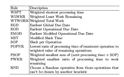
The following heuristics are used for dynamic JSSPs:
For example, a chromosome can be represented with (
m, h) where,
- m = 0 1 01 1 1 0 0 ..... (method numbers)
- h = 0 12 8 9 2 0 4 7 1 0 3 5 5
.... (the heuristic numbers for the above heuristics)
This representation guarantees a feasible solution and recombination
operators can produce feasible offsprings.
The objectives functions used in HGA are four
normalized weighted
objective functions:

where,
- ETwt: Weighted Earliness plus Tardiness,
- Fwt: Weighted Flowtime,
- Lwt: Weghted Lateness,
- Twt: Weighted Tardiness.
- Cj: completion time of job j,
- rj: arrival time of job j,
- Ej: earliness, as max (-Lj,
0),
- Lj: lateness, as (Cj
- Dj), Dj is the duetime of job
j,
- Tj: max of (Lj, 0).
2.4 Case-Injected Genetic AlgoRithm (CIGAR)
Case-injected GA uses the similar method as case-based reasoning (CBR)
in which the cases (old problems and solutions) helps solve a
new problem which is similar to the old one. According to [1], a case
in GA is member of the population (for example, a schedule in JSSP) together
with other information such as fitness, the generation this case was generated,
and its parent. The process of using case-injected GA for a certain
problem can be described as: 1). define and create similar problems, 2).
build up case-base, and 3). case-injected GA search.
Our starting point is that similar problems have similar solutions. In
GAs, solutions are encoded as strings and [1] shows that "purely syntactic
similarity measures lead to surprisingly good performance." Hamming distance
and Longest Common Subsequence (LCS) can used to express the similariy.
For two sequences of strings with same length, Hamming distance between these
two is the number of symbols that disagree. The less this number, the more
similar the two sequences. As in LCS, the longer the LCS the more similar
the two encoded solutions.
In case of our JSSP, for a certain JSSP, a similar problems can be
generated by modifying a randomly picked set of tasks (40% of all the tasks)
and changing the picked task's duration by a randomly picked amount
upto 20% of the maximum duration of a task. 50 similar problems are used
to build up the case-base.
For each of the 50 similar problems, we run the HGA. In every generation
during GA search, if the the fitness of the best individual increases, this
new best individual will be stored in the case-base.
When dealing with the JSSP, we inject a small number of cases as part of
the initial population and randomly produce the other part of the population.
From then on during GA's evolution we periodically (every 5 generations
in our experiment) inject into the current population some solutions (cases)
that are similar to the current best member of the GA population (using
Hamming distance method as similarity metric).
It is advised to refer to [1] for specific description of CIGAR system and
its application.
2.5 CIGAR-incorporated HGA
CIGAR-incorporated HGA can be considered as
a specific (smply) application
of CIGAR. It follows nearly all the steps proposed in [1] except that
in our experiment we only used Hamming distance for measuring similarity
and used 25 similar problems. HGA method replaced the GA search process.
3. Experiments and Results
We tested the CIGAR-incorporated HGA on 20x15 and 15x3 dynamic JSSPs
which are:
- 20x15.ss: job-machine (static ) jssp,
- 20x15.ww: job's duetime/arrivaltime/weightness
for above 20x15 jssp,
- jb9.ss: a 15x3 job-machine (static) jssp,
- jb9.ww: the above 15x3's duetime/arrivaltime/weightness
the 15x3 jssp.
The GA parameters used are: population, 200; generation ,100. 25 similar
problems are created for building up case-base. The
method allele
is mutted with probability of 0.5, and
heuristic allele's is 0.01.
Generational reproduction strategy with rank selection is used. The program
runs for 10 times to get the final average results. The results are
normalized
as did in HGA [3] for comparison (at first, we produced makespans for
some runs to examine the correctness of the results).
Following tables are sampled results for the earliest 20 generations. The
detailed results are in the graphs thereafter. Here in the table and graph,
HGA means results from HGA method and CIGAR the results from CIGAR-incorporated
HGA method. The results from HGA method were from our implementation output
not from [3].
Generation
|
0
|
2
|
4
|
6
|
8
|
10
|
12
|
14
|
16
|
18
|
HGA
|
0.43199
|
0.39424
|
0.38855
|
0.38798
|
0.38798
|
0.38798
|
0.38798
|
0.38798
|
0.38798
|
0.38798
|
CIGAR
|
0.38392
|
0.37735
|
0.37645
|
0.37645
|
0.37645
|
0.37645
|
0.37645
|
0.37645
|
0.37645
|
0.37645
|
Table 1. EW15x3(Weighted earliest + Tardiness for
15x3 D-JSSP)
Generation
|
0
|
2
|
4
|
6
|
8
|
10
|
12
|
14
|
16
|
18
|
HGA
|
1.8271
|
1.7795
|
1.7706
|
1.77
|
1.7687
|
1.7687
|
1.7687
|
1.7687
|
1.7687
|
1.7687
|
CIGAR
|
1.7845
|
1.7677
|
1.7665
|
1.7658
|
1.7652
|
1.7652
|
1.7652
|
1.7652
|
1.7638
|
1.7638
|
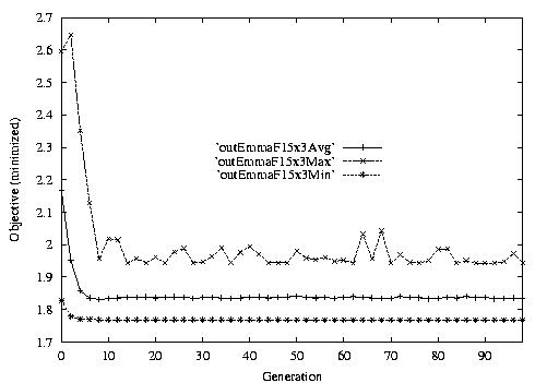
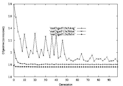
Table 2. F15x3(Weighted Flow Time for 15x3 D-JSSP)
Generation
|
0
|
2
|
4
|
6
|
8
|
10
|
12
|
14
|
16
|
18
|
HGA
|
0.00079
|
-0.0391
|
-0.0547
|
-0.0576
|
-0.0576
|
-0.0576
|
-0.0576
|
-0.058
|
-0.058
|
-0.058
|
CIGAR
|
-0.0574
|
-0.0648
|
-0.0669
|
-0.0669
|
-0.0669
|
-0.0669
|
-0.0669
|
-0.0669
|
-0.0672
|
-0.0672
|
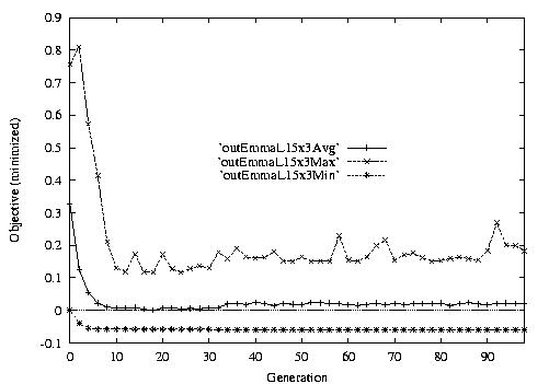
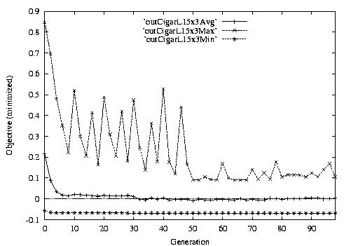
Table 3. L15x3(Weighted Lateness for 15x3 D-JSSP)
Generation
|
0
|
2
|
4
|
6
|
8
|
10
|
12
|
14
|
16
|
18
|
HGA
|
0.243
|
0.1957
|
0.1914
|
0.1914
|
0.1914
|
0.1914
|
0.1914
|
0.1914
|
0.1914
|
0.1914
|
CIGAR
|
0.1819
|
0.1771
|
0.1771
|
0.1762
|
0.17540
|
0.1754
|
0.1754
|
0.1754
|
0.1754
|
0.1754
|
Table 4. T15x3(Weighted Tardinessfor 15x3 D-JSSP)
Generation
|
0
|
2
|
4
|
6
|
8
|
10
|
12
|
14
|
16
|
18
|
HGA
|
0.1688
|
0.1501
|
0.1399
|
0.1299
|
0.1272
|
0.1263
|
0.1258
|
0.1248
|
0.1248
|
0.1248
|
CIGAR
|
0.1542
|
0.1403
|
0.1327
|
0.1253
|
0.1244
|
0.1243
|
0.1241
|
0.1238
|
0.1238
|
0.1238
|
Table 5. EW20x15(Weighted earliest + Tardiness
for 20x15 D-JSSP)
Generation
|
0
|
2
|
4
|
6
|
8
|
10
|
12
|
14
|
16
|
18
|
HGA
|
1.4063
|
1.3916
|
1.3837
|
1.3775
|
1.3766
|
1.3741
|
1.3739
|
1.3736
|
1.3734
|
1.3731
|
CIGAR
|
1.3895
|
1.3732
|
1.3682
|
1.3624
|
1.3603
|
1.3584
|
1.3581
|
1.357
|
1.357
|
1.357
|
Table 6. F20x15(Weighted Flow Time for 20x15 D-JSSP)
Generation
|
0
|
2
|
4
|
6
|
8
|
10
|
12
|
14
|
16
|
18
|
HGA
|
0.2573
|
0.0064
|
-0.0105
|
-0.0214
|
-0.0238
|
-0.0267
|
-0.0267
|
-0.0267
|
-0.0267
|
-0.0267
|
CIGAR
|
-0.0036
|
-0.0202
|
-0.029
|
-0.0303
|
-0.0322
|
-0.0328
|
-0.0332
|
-0.0332
|
-0.0332
|
-0.0332
|
Table 7. L20x15(Weighted Lateness for 20x15 D-JSSP)
Generation
|
0
|
2
|
4
|
6
|
8
|
10
|
12
|
14
|
16
|
18
|
HGA
|
0.1051
|
0.0918
|
0.0873
|
0.0816
|
0.0795
|
0.079
|
0.079
|
0.079
|
0.079
|
0.079
|
CIGAR
|
0.1011
|
0.0942
|
0.0855
|
0.0831
|
0.0814
|
0.0782
|
0.0779
|
0.0779
|
0.0779
|
0.0779
|
Table 8. T20x15(Weighted Tardinessfor 20x15 D-JSSP)
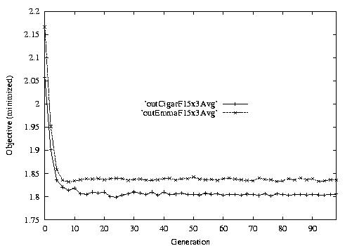
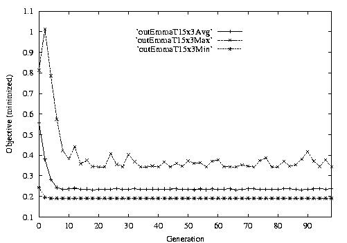
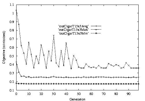
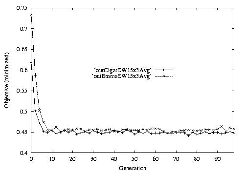
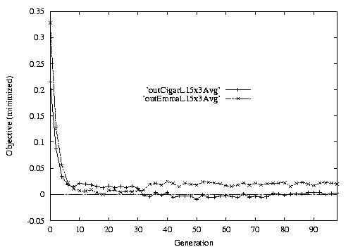
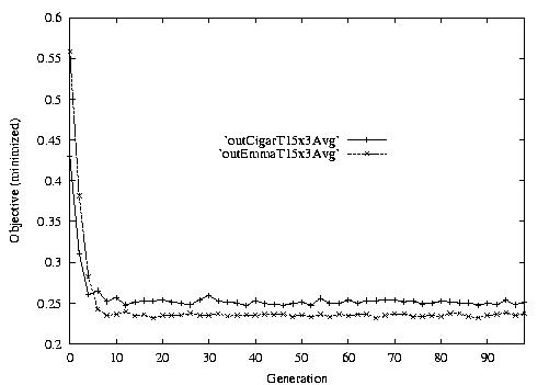
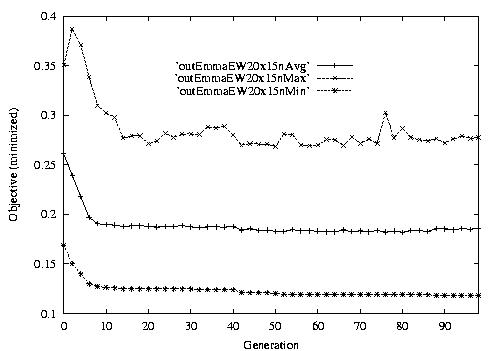
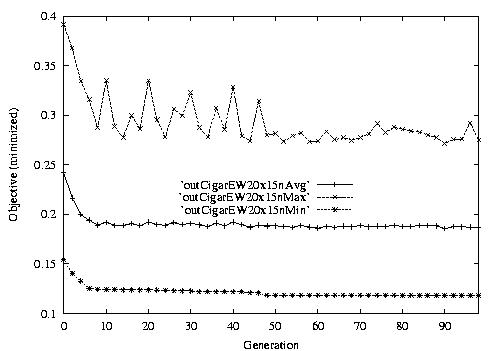
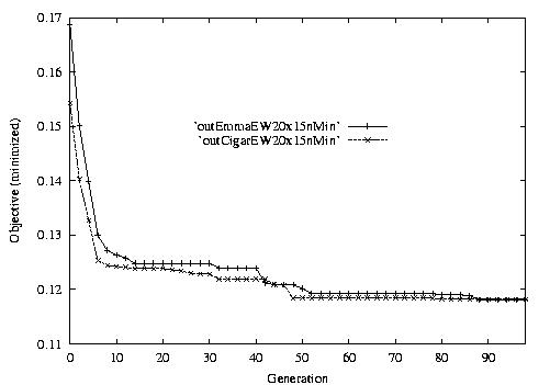
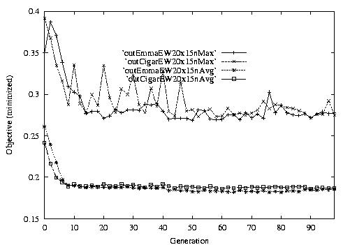
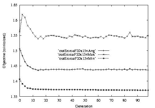
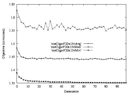
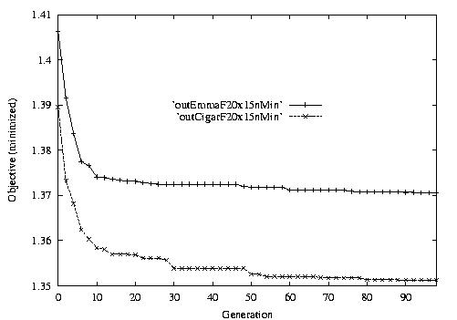
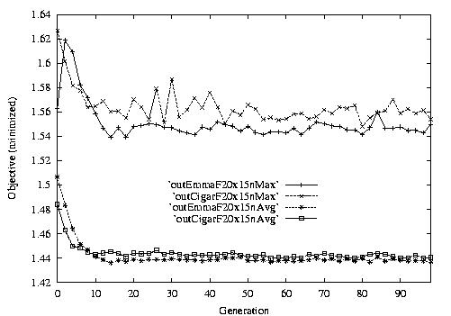
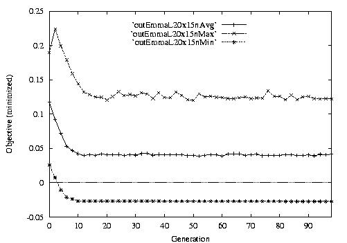
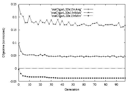
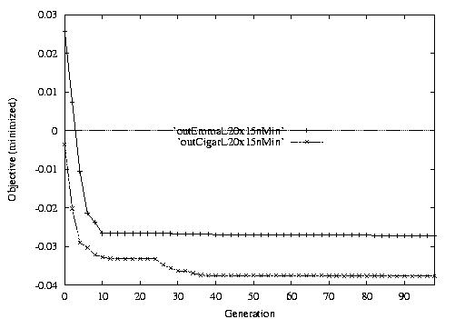
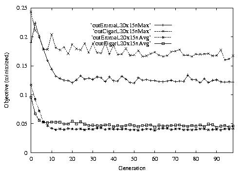
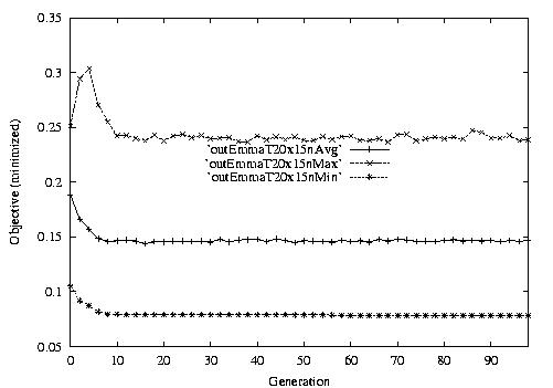
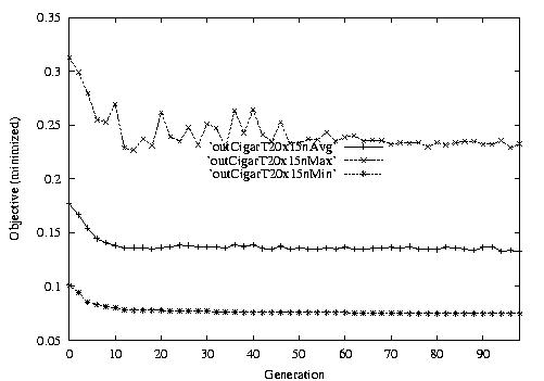
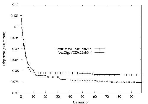
Following are the result graphs. The legends in the diagrams are self-explained:
- emma: HGA results,
- cigar: case-ingected HGA results,
- 20x15 or 15x3: the dynamic JSSPs,
- EW: Earliest plus Tardiness objective function,
- T: Tardiness objective function,
- L: Lateness objective function,
- F: Flow time objective function,
- n: ignore this, type error,
- Avg: averaged objective for the whole population at a generation,
- Min: the best objective for the whole population at a generation,
- Max: the worst objective for the whole population at a generation.
For example, in the following diagram,
we interpret it as: for 15x3 D-JSSP, their average performance in 100
generations. The objective function is "F"---the normalized minimum flow
time (in every generation).
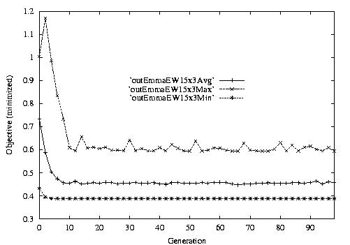
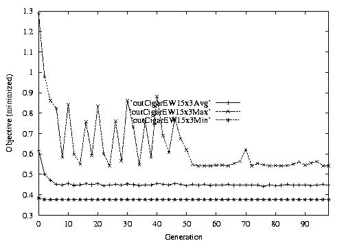
3.1 15x3 D-JSSP
Fig. 1. HGA / CIGAR performance on EW15x3